A network is more than just a collection of connected objects. It is a system through which something can move, spread, and interact. So, understanding how information travels through networks is really about understanding how these connections shape its journey.
You know how a signal fires from one neuron and, a few synapses later, it becomes a thought. How a text message hops across cell towers and fiber-optic cables to reach your friend. And how your delivery partner picks up your order from the warehouse and reaches your location almost successfully every time.
All these systems seem completely different but they share a common skeleton: nodes connected by edges, through which information/data travels. The interesting question is therefore not simply what is connected to what?, but: What Does It Mean for Information to Travel Through a Network? How Does Information Find Its Way Through a Network? How Efficiently Can Information Move Across a Network? How Does Information Spread Through a Network? How Does Machine Learning Learn From Information Moving Through a Network?
We are going to take each question step by step and explore how the same fundamental ideas appear across computer networks, biological neural networks, and machine learning models. Along the way, we will see how concepts such as paths, diffusion, efficiency, propagation, and message passing give us a common language for understanding how information moves through complex systems.
What Does It Mean for Information to Travel Through a Network?
Before we understand the traversal of information through a web of network, let us understand the structure of a network.
A network is basically a system made up of entities and the relationships or connections between them. Mathematically, a network is represented as a Graph. Each entity is a node. In computer science, a node can be a router, a computer, a webpage, or maybe a user. Whereas, each relationship/connection is an edge between the two nodes. Now, a path of a network can follow a direction and stay along that designated direction, these will be our Directed Graphs. While, some networks are independent of any direction, i.e., the information can travel both forward or backward through a path. These are represented using Undirected Graphs.
Now that we have basic building blocks of a network: nodes, edges, and direction in which those edges allow information to travel, we can now start looking for ways in which an information can travel. Simplest structure is Direct Communication. Here, two nodes are directly connected by an edge. So, information can easily traverse from node A to node B.
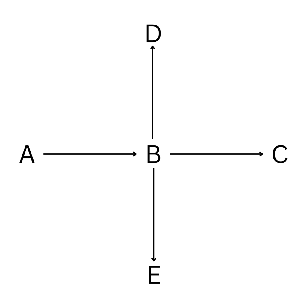
But, what about when A want to share information with C? Then it has to go through B. This is called Indirect communication through intermediate nodes. This brings us to the idea of a Neighbourhood. The nodes directly connected to a particular node are its neighbours. For example, if B is connected to A, C, D, and E, then these nodes form B’s neighbourhood. In simple terms, a node’s neighbours tell us where information can go next. This is important because information moving through a network is essentially a sequence of these local steps, from one node to its neighbour, then to another neighbour, and so on. Once multiple such steps are combined, they form a path through the network.
Before we move forward, let us look at a few simple ways to represent the same network. These representations do not change the network; they simply make its connections easier to see, organize, and work with.
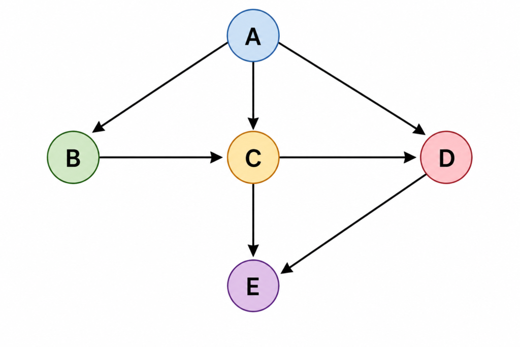
Consider this network:
Adjacency Matrix
An adjacency matrix represents all the connections of a network in a table. 1 means that a direct connection exists between two nodes, while 0 means there is no direct connection.
\begin{array}{c|ccccc}
& A & B & C & D & E\\
A & 0 & 1 & 1 & 1 & 0 \\
B & 0 & 0 & 1 & 0 & 0\\
C & 0 & 0 & 0 & 1 & 1\\
D & 0 & 0 & 0 & 0 & 1\\
E & 0 & 0 & 0 & 0 & 0
\end{array}
For example, the 1 in the row A and column B tells us that information can travel directly from A to B.
Degree of a Node
The degree tells us how many direct connections a node has. In our network, A has three outgoing connections- to B, C, and D, so its out-degree is 3.
Edge Weights
Sometimes, a connection has more information than simply “connected” or “not connected.” An edge weight assigns a number to a connection to represent something such as distance, time, cost, or strength. For example, if travelling from A to B takes 5 ms, we can give the edge A → B a weight of 5.
Together, these representations help us turn a network into something that is easier to analyze mathematically, which becomes important when we start studying how information moves through it.
How Does Information Find Its Way Through a Network?
Now that we are well equipped with the basic structure and representation of a network, we can ask the next question: if information has to travel from one node to another, what route can it take? Imagine information starting at A and trying to reach D. There may be more than one way to get there, and before we decide which one is better, we first need a way to describe these routes.
A sequence of nodes through which information travels is called a walk. For example, \(A \rightarrow B \rightarrow C \rightarrow D\) is a walk through the network. When we consider a route without repeating nodes, we call it a path. The number of edges information crosses along this path is its path length, also commonly called the number of hops. Here, \(A \rightarrow B \rightarrow C \rightarrow D\) has 3 hops.
Now, if there are multiple paths between A and D, which one should we choose? Often, we are interested in the shortest path, which is, the route that requires the fewest hops in an unweighted network or the lowest total cost in a weighted one. For example, if one route takes 3 hops and another takes 5, the first is the shorter path. If the edges have weights representing distance or time, however, we compare the total weight of each route instead.
Once we know what kind of route we are looking for, we can use different algorithms to find it. Breadth First Search(BFS) is commonly used to find shortest paths in an unweighted network, Dijkstra’s algorithm works when edge weights are non-negative, Bellman–Ford can handle negative edge weights, and Floyd–Warshall finds shortest paths between all pairs of nodes. The algorithms differ, but they are all solving the same broader problem: finding efficient routes through a network. You can read more about these algorithm here. Or you can wait for a while I am soon planning to cover these topics myself😬.
We can also step back from individual routes and ask how well the entire network is connected. The average shortest-path length tells us how many steps are typically needed to travel between nodes, while the network diameter tells us the longest of these shortest paths. Global efficiency gives us another way to describe how efficiently information can travel across the network as a whole.
This idea is useful far beyond a simple graph. In computer science, shortest-path analysis helps us understand routes through the internet, communication networks, and transportation systems. In computational neuroscience, we can treat brain regions as nodes and their structural connections as edges, then use shortest paths to characterize how closely or distantly different regions are connected. This does not mean that the brain necessarily chooses the shortest path; rather, shortest-path analysis provides a mathematical measure of potential communication efficiency.
How Efficiently Can Information Move Across a Network?
So far, we have seen that information can travel through paths, and that when multiple paths exist, we can look for the shortest one. But here is something interesting: having a path does not necessarily mean having an efficient network. Two networks can have the same number of nodes and connections, yet information may move much more easily through one than the other. Why? Because where those connections are placed matters.
Imagine two people trying to reach the same destination. One has a direct road, while the other has to take several turns and detours. Both can reach the destination, but one journey is clearly more efficient. Networks work in much the same way. We have two types of efficiencies: Global efficiency looks at how easily information can travel between different parts of the entire network, while local efficiency looks at how well a small neighbourhood remains connected when we focus on it.
And here enters, something called Network Topology. A network topology is the overall arrangement of connections in a network. We already know that the degree tells us how many connections a node has. But what happens when we look at the degrees of all the nodes? That gives us the degree distribution. Similarly, density tells us how many of the possible connections actually exist, while the clustering coefficient tells us how strongly a node’s neighbours are connected to one another.
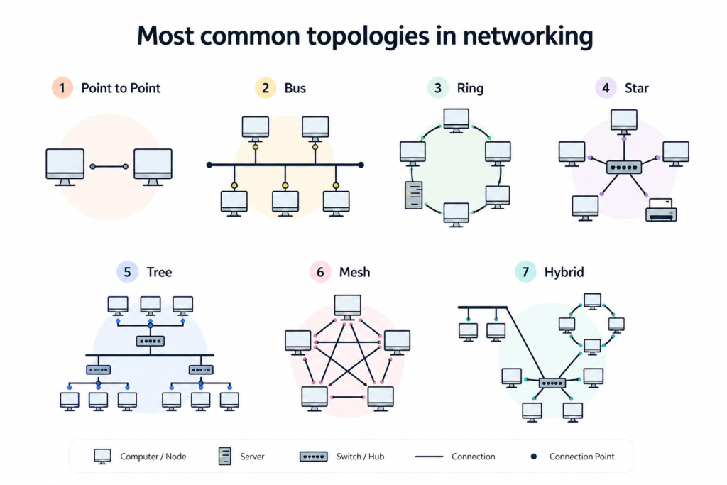
In the above diagram, we can observe that some nodes begin to stand out. A few may have far more connections than the others. These are hubs. Because so many connections meet at a hub, it can act like a busy intersection, allowing information to reach many parts of the network more easily. But this also makes the network vulnerable: if an important hub fails, communication across several regions can be disrupted. Sometimes, however, the most important connection is not a highly connected node. It can be a single link connecting two otherwise separate parts of the network. These connections act as bridges. When a large amount of information has to pass through a small number of such connections, they can become bottlenecks, restricting how efficiently information can move between different regions.
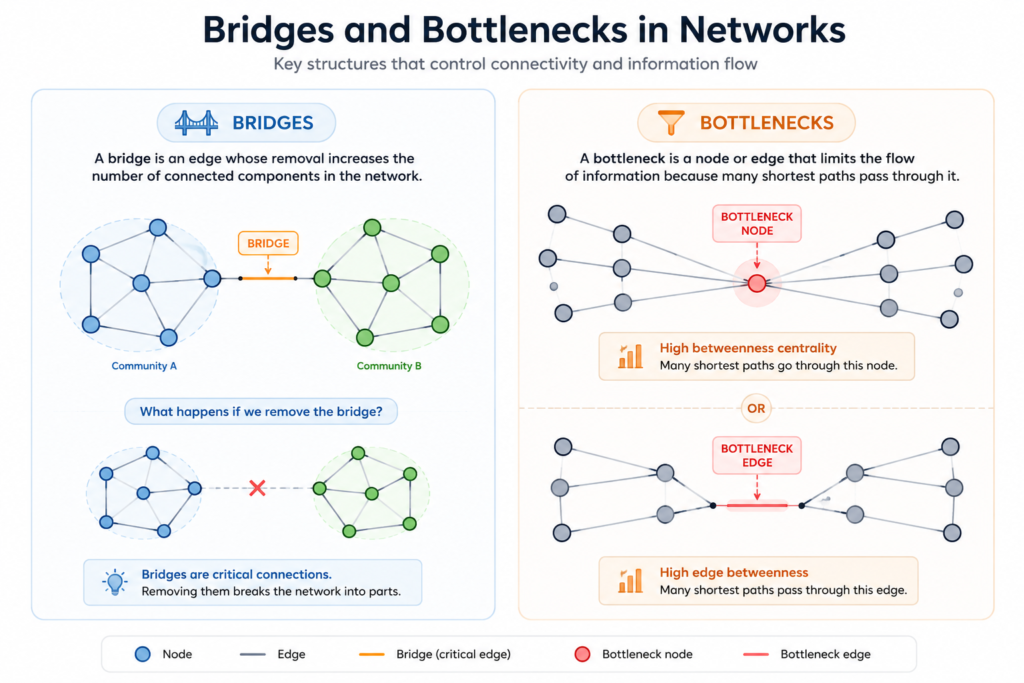
Now imagine that we add just one connection between two distant parts of the network. Suddenly, a journey that required several steps might become much shorter. These long-range connections act as shortcuts. When a network combines tightly connected local neighbourhoods with a few such shortcuts, it can form what is known as a small-world network, allowing information to move efficiently across the network while still maintaining strong local connections. But networks are not always one big, uniformly connected structure. Often, they naturally break into groups where nodes are highly connected to one another but have fewer connections outside the group. These are communities or modules. Information can move easily within a community, while communication between communities may depend on a few bridges. This balance between local interaction and global communication is one of the most interesting features of complex networks.
How Does Information Spread Through a Network?
So far, we have been following information as if it were travelling somewhere: from A to B, choosing a path, perhaps even finding the shortest one. But information does not always behave like a traveller with a destination. Sometimes, it spreads. One node passes something to its neighbours, those neighbours pass it further, and before we know it, activity that started in one small corner of the network has reached much farther than where it began. Just like a rumour, you tell one person, they tell two more, and suddenly half the network somehow knows.
This is where we need to make a small but important distinction. Routing is about choosing a particular path: \(A \rightarrow B \rightarrow C \rightarrow D\). Diffusion is different. Instead of choosing one route, information or activity can propagate from A to several of its neighbours at once. Those neighbours can then pass it to their neighbours, allowing a local event to gradually become a network-wide phenomenon.
Imagine A becomes active. It influences B and C. Now B and C can influence the nodes around them, and the process continues:
\[
A \rightarrow {B,C} \rightarrow {D,E,F,\ldots}
\]
What happens next depends heavily on the structure of the network. In a densely connected region, activity can spread quickly because there are many possible connections. In a sparse region, it may move much more slowly, or stop altogether. A hub can suddenly accelerate the spread, while a tightly separated community can keep it largely contained.
One way to understand this movement is through a random walk. Imagine a person standing at node A, randomly choosing one of its neighbouring nodes, then choosing another neighbour from there, and continuing this journey. If we repeat this process many times, we start to see patterns in where movement tends to accumulate. This simple idea connects naturally to diffusion: repeated local movement can gradually reveal how activity flows through the larger network.
We can even represent these movements mathematically using a transition matrix, where the entries describe the probability of moving from one node to another. Instead of asking “Which path will information take?”, we are now asking something slightly different: “How likely is information or activity to move from here to there?”
And this is where the structure of the network starts meeting mathematics more directly. The graph Laplacian gives us a way to mathematically describe how something can flow or diffuse across a network:
\[
L = D-A
\]
Here, \(A\) is the adjacency matrix, which tells us how nodes are connected, and \(D\) is the degree matrix, which tells us how many connections each node has. The Laplacian essentially captures the difference between what is happening at a node and what is happening around it, making it a useful tool for studying diffusion on graphs.
We can take this one step further through the eigenvalues and eigenvectors of the Laplacian. Without getting buried in the linear algebra, the important idea is that they carry information about the structure of the network and help us understand how quickly and in what patterns activity can spread through it.
Now imagine this process happening not just once, but repeatedly. A message gets shared, a rumour reaches a few people who pass it on, or a piece of content suddenly goes viral. What started as a small local event becomes a cascade.
Sometimes the spreading remains inside one community. Sometimes it crosses a bridge and reaches another community. And sometimes a highly connected hub gives it the push it needs to travel across a huge portion of the network. The same basic mechanism can describe very different phenomena, from disease spreading through populations to information spreading through social networks.
How Does Machine Learning Learn From Information Moving Through a Network?
If the structure of a network determines how information can move, can a machine-learning model learn from that structure? This is where everything we have discussed so far starts coming together. A Graph Neural Network (GNN) represents data as a graph, where nodes can represent things like people, webpages, or brain regions, and edges represent the relationships between them. Nodes and edges can also carry additional information, such as features describing a brain region or the strength of a connection. Instead of looking at each node in isolation, the model looks at its neighbourhood and learns from the information flowing through these connections.
The basic idea is surprisingly simple: Node → Neighbours → Aggregate → Update. A node receives information from its neighbours, combines it, and updates its own representation. After one round, it has information from its 1-hop neighbours; after two rounds, information can reach from the 2-hop neighbourhood, and so on. Remember our earlier discussion about paths? If A and D are three hops apart, information from A generally needs multiple rounds of message passing to influence D. Different GNN architectures, such as GCN, GraphSAGE, GAT, and GIN, approach this neighbourhood aggregation in slightly different ways, but the underlying idea remains the same: learn from both the data and the structure connecting the data.
And suddenly, all the pieces of our journey fit together. Nodes become data entities, edges become relationships, neighbourhoods provide local information, paths and hops describe how far information needs to travel, diffusion resembles repeated information propagation, and hubs and communities shape where that information can move easily or become restricted. The network is no longer just something we analyse, it becomes part of what the model learns from. And that is what makes graph-based learning so interesting: the connections between things are not merely the background; they are part of the information itself.
And that’s where I’ll leave our little journey through networks. If you enjoyed seeing how information moves through paths, communities, and eventually into Graph Neural Networks, you might want to take the next step and see what happens when these ideas meet the mathematics underneath machine learning. You can continue that journey here: Why Linear Algebra Runs Machine Learning.
And now, if you made it this far, I’m genuinely curious: did this article make networks feel a little less intimidating and a little more interesting? If something clicked for you, or there was a moment where you thought “wait… I never looked at it that way”, tell me about it. And if something felt confusing, unnecessarily complicated, or just plain boring, I want to hear that too. You can be honest, I promise the network won’t route your feedback through three intermediate nodes before it reaches me. 😄