These “non-numerics” are often referred to as Categorical Features in machine learning.
Almost every feature set we use for our ML model contains some categorical features that have the potential of becoming great predictors, but, because the model can only work with numerics, they often go underused. Encoding in machine learning give us a way to bring them into the picture by turning them into numerical features that the model can actually learn from.
Before diving into encoding, it helps to understand what categorical features actually are, the different types we encounter, and why we can’t simply feed them to a model as they are.
As I mentioned earlier, these “non-numerics” are what we call categorical features in machine learning. They represent groups or categories rather than numerical quantities, for example, city, blood type, product category, or education level. Depending on whether these categories have a meaningful order or not, categorical features are generally divided into two types: nominal and ordinal. Nominal features are categories with no inherent order, while ordinal features have a meaningful ranking or order between their categories.
There is one more thing that matters when we work with categorical features: how many different categories does the feature actually contain? This is known as its cardinality. A feature like blood type has only a handful of possible values, so it has low-cardinality. A feature like city, on the other hand, could contain hundreds or even thousands of unique values. When a categorical feature has a very large number of unique values, we call it high-cardinality. This becomes important when choosing how to encode the feature, because some encoding methods can create a huge number of new features when there are too many categories.
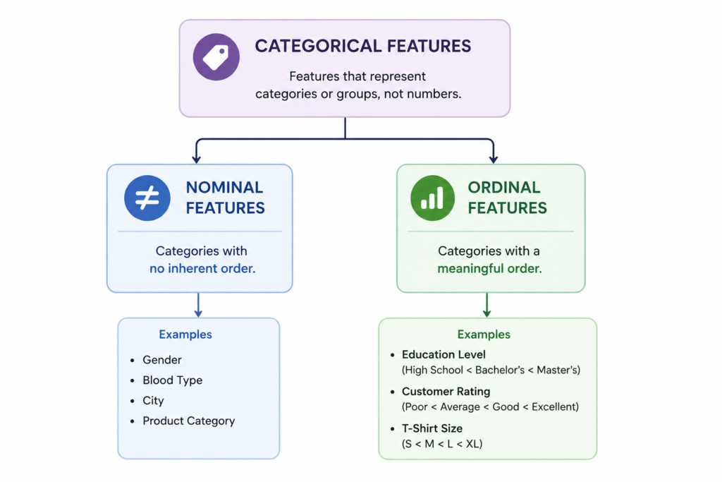
The important part is that these categories carry information, even though they are not numbers, they are fully capable of influencing the prediction. For example, a city can tell us something about a customer because people from the same city may share certain characteristics, such as local preferences, lifestyle, income patterns, or access to particular products and services. The problem is that the model cannot directly make sense of these labels. We need a way to translate the information hidden in these categories into numbers without losing what makes them meaningful. This is exactly what encoding helps us do.
Encoding in Machine Learning
Encoding is the process of converting categorical values into numerical representations that can be used as features by a machine learning model. But there is no single way to do this. The right approach depends on the type of categorical feature and, more importantly, on the kind of relationship its categories have with one another.
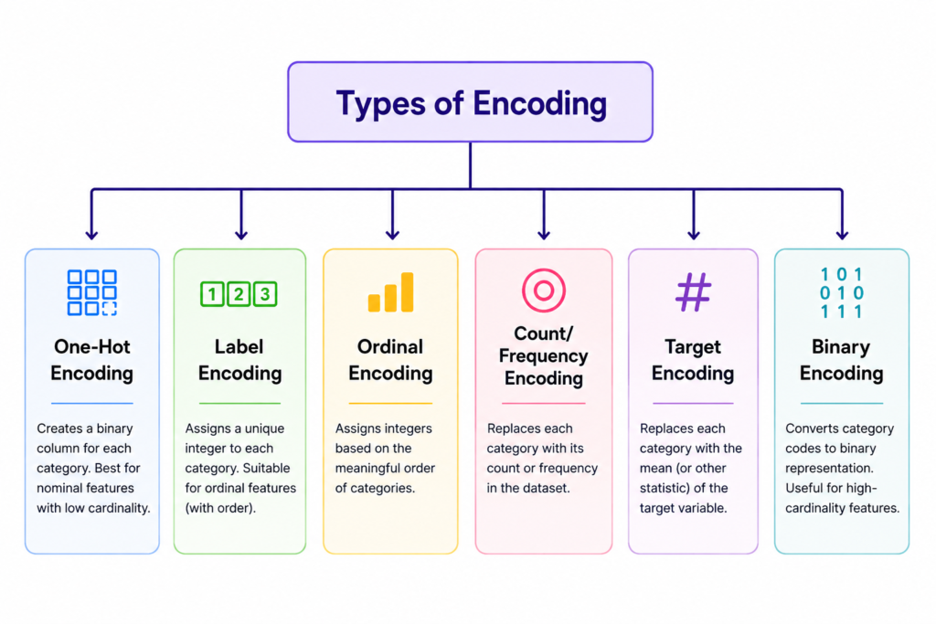
Let us start with the simplest encoding technique.
Label Encoding
Suppose we have a City feature with three values: Delhi, Mumbai, and Bangalore. We could simply assign each category a number:
| City | Encoded Value |
|---|---|
| Delhi | 0 |
| Mumbai | 1 |
| Bangalore | 2 |
This is Label Encoding. Each category is assigned a unique integer. In Python, this can be done using LabelEncoder:
from sklearn.preprocessing import LabelEncoder

encoder = LabelEncoder()

df["city_encoded"] = encoder.fit_transform(df["city"])
Reasonable, right? Well, there IS a problem. By assigning Delhi = 0, Mumbai = 1, and Bangalore = 2, we have unintentionally introduced an order that does not actually exist. The model might interpret Bangalore as being “greater than” Mumbai, which makes no sense.
Label encoding therefore needs to be used carefully. It makes much more sense when the categories themselves have a meaningful order.
And that brings us to Ordinal Encoding.
Ordinal Encoding
Ordinal encoding is built around one simple idea: the order between categories matters. Consider a feature such as Customer Satisfaction, it has a specific order, say, Poor → Average → Good → Excellent. Here, the order actually means something. We can represent it as:
| Satisfaction | Encoded Value |
|---|---|
| Poor | 0 |
| Average | 1 |
| Good | 2 |
| Excellent | 3 |
Unlike Delhi, Mumbai, and Bangalore, these categories are not just different labels. There is a meaningful progression from Poor to Excellent. Assigning numbers in that order allows the model to retain that information. The important thing here is not the numbers themselves. The numbers are useful because they represent a relationship that already exists in the data.
Using OrdinalEncoder, we can explicitly tell Python what that order is:
from sklearn.preprocessing import OrdinalEncoder

encoder = OrdinalEncoder(
    categories=[["Poor", "Average", "Good", "Excellent"]]
)

df["satisfaction_encoded"] = encoder.fit_transform(
    df[["satisfaction"]]
)
But what if the categories don’t have any meaningful order?
For that, one-hot encoding is usually a better fit.
One-Hot Encoding
Let’s go back to our City feature. Delhi, Mumbai, and Bangalore are simply different categories. There is no meaningful ranking between Delhi, Mumbai, and Bangalore. So instead of forcing them onto a numerical scale, we can give each category its own feature:
| City | Delhi | Mumbai | Bangalore |
|---|---|---|---|
| Delhi | 1 | 0 | 0 |
| Mumbai | 0 | 1 | 0 |
| Bangalore | 0 | 0 | 1 |
This is One-Hot Encoding. Each category gets its own column, and a value of 1 indicates that the observation belongs to that category. Everything else is 0. Now there is no accidental ranking. Delhi is not smaller than Mumbai, and Bangalore is not greater than either of them. They are simply separate categories. This makes one-hot encoding a natural choice for many nominal features.
from sklearn.preprocessing import OneHotEncoder

encoder = OneHotEncoder(
    sparse_output=False,
    handle_unknown="ignore"
)

encoded = encoder.fit_transform(df[["city"]])
There is one obvious downside, though. Here, a City feature has only 3 categories. Three new columns are manageable. But what if it contains 5,000? Now one feature has exploded into 5,000 columns, increasing the size of our dataset and making the model’s job unnecessarily complicated. This brings us back to the idea of cardinality.
Frequency/Count Encoding
When a categorical feature contains a large number of unique values, creating a separate column for every category may not be practical. Instead of representing which category something belongs to, we can sometimes represent how often that category appears in the dataset.
This is the basic idea behind Count Encoding or Frequency Encoding. Suppose our dataset contains:
| City | Count |
|---|---|
| Delhi | 500 |
| Mumbai | 300 |
| Bangalore | 150 |
| Jaipur | 50 |
We could replace the city with its count:
| City | Encoded Value |
|---|---|
| Delhi | 500 |
| Mumbai | 300 |
| Bangalore | 150 |
| Jaipur | 50 |
This can be surprisingly useful for high-cardinality features because it gives us one numerical feature instead of hundreds or thousands of new columns.
In Python:
frequency = df["city"].value_counts()

df["city_frequency"] = df["city"].map(frequency)
Now one feature remains one feature, regardless of how many cities we have.
Frequency encoding is particularly useful when the fact that a category is common or rare carries information. But it does not tell the model what the category actually is.
Sometimes, what matters is how a category relates to the target we are trying to predict.
But notice what we have done: we are no longer telling the model which city it is. We are telling it how common that city is in the dataset. Whether that is useful depends entirely on the problem.
And sometimes, frequency is not what matters at all. What we really care about is how a category relates to the target we are trying to predict.
That leads us to target encoding.
Target Encoding
Suppose we are predicting whether a customer will purchase something. We have a categorical feature called City. Instead of simply counting how often each city appears, we can look at the average target value for each city. We might find that customers from Delhi have a purchase rate of 72%, while customers from Mumbai have a rate of 58%.
We can represent the city using these target-related values:
| City | Purchase Rate |
|---|---|
| Delhi | 0.72 |
| Mumbai | 0.58 |
| Bangalore | 0.41 |
We can replace each city with its corresponding value. So a customer from Delhi gets 0.72, Mumbai gets 0.58, and Bangalore gets 0.41. This is what behind Target Encoding looks like, the category is represented using information derived from the target variable. And this can be powerful. If customers from one city consistently have a higher probability of making a purchase, target encoding gives the model a way to capture that relationship without creating a separate column for every city.
In Python, Target Encoding can be achieved using this snippet:
target_mean = df.groupby("city")["purchased"].mean()

df["city_target_encoded"] = df["city"].map(target_mean)
But the problem here is: We are using the target to create a feature that will then be used to predict that same target. If we calculate these values carelessly, information from the target can leak into the features and make the model look much better than it really is. So target encoding needs to be done carefully, usually with techniques such as smoothing and out-of-fold encoding, especially when working with small or high-cardinality categories.
Binary Encoding
There is another way to deal with high-cardinality categorical features: Binary Encoding.
The basic idea is quite simple. Instead of creating one column for every category, we first assign each category a number and then represent that number in binary. For example:
| Category | Number | Binary |
|---|---|---|
| Delhi | 1 | 001 |
| Mumbai | 2 | 010 |
| Bangalore | 3 | 011 |
| Lucknow | 4 | 100 |
The binary digits are then split into separate columns. The result is a representation that usually needs far fewer columns than one-hot encoding. That can make a big difference when the number of categories gets large. We can implement binary encoding in python:
import category_encoders as ce

encoder = ce.BinaryEncoder(cols=["city"])

df_encoded = encoder.fit_transform(df)

print(df_encoded)
Of course, binary encoding is not automatically better. Like every encoding technique, it introduces its own representation of the categories, and whether that representation works well depends on the model and the data.
So, Which One Should You Use?
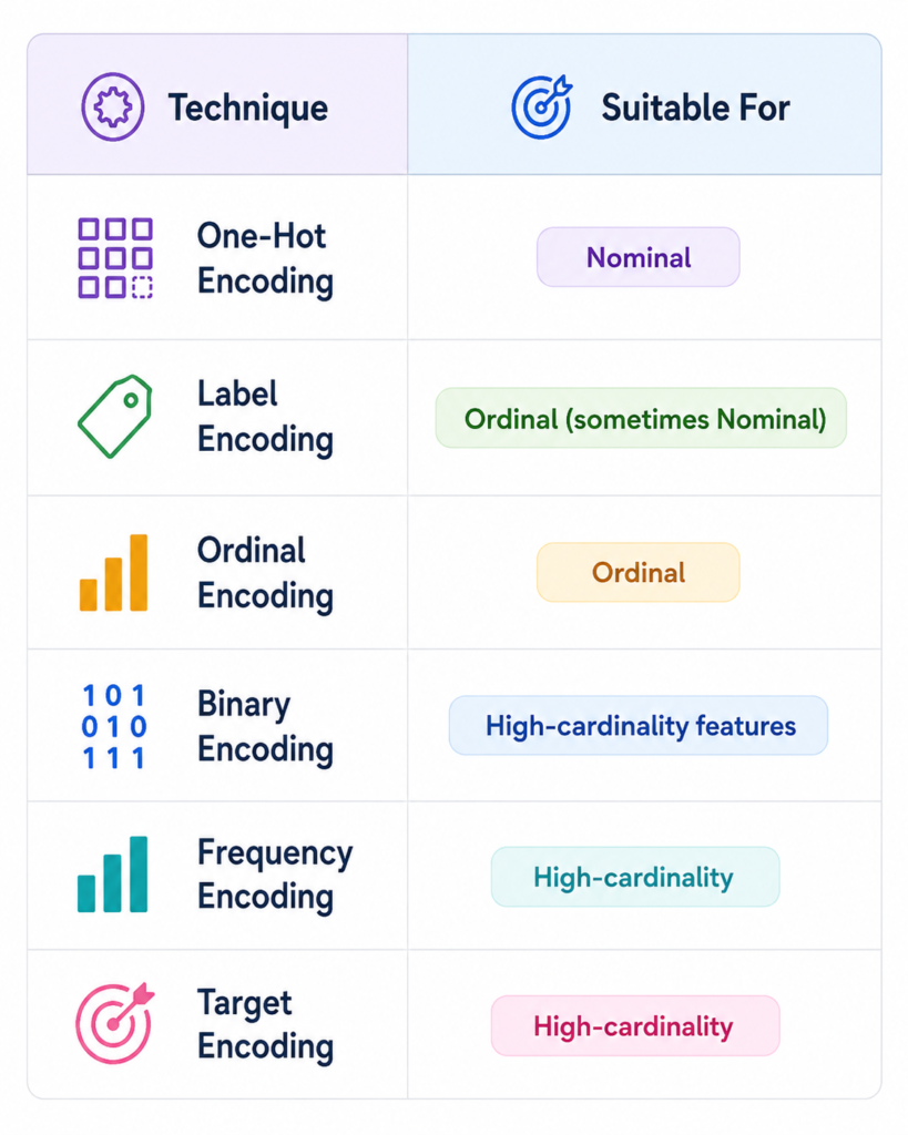
There is no single encoding technique that works best for every categorical feature. The right choice depends on what the categories mean, how many of them there are, and how the model is going to use the resulting numbers. For a small nominal feature such as blood type, One-Hot Encoding is often a straightforward choice. For something ordered, such as Poor → Average → Good → Excellent, Ordinal Encoding can preserve the ranking. For a feature with hundreds or thousands of categories, one-hot encoding may become expensive, so methods such as Frequency, Target, Binary, or other high-cardinality encoders may be worth considering.
The key is to think about the information contained in the original feature before choosing how to represent it. After all, encoding is not really about turning words into numbers. It is about deciding what those numbers should mean. And that distinction will decide the future of you machine learning model.
And this is only one small piece of the much bigger world of machine learning. I genuinely love learning how these models work—not just the how, but the why behind them. The more I learn, the more fascinating I find the connection between data, computation, and the way we understand intelligence itself.
If you’re continuing your ML journey, you can explore my other articles on Machine Learning, Data Science, and Computational Neuroscience on my website.
And if you’re curious about the things I’m learning, building, and obsessing over along the way, come explore the rest of my blog. There’s always another concept to unpack, another paper to read, or another question about the brain that makes me go down a three-hour research rabbit hole.
Oh I almost forgot, here are few links where you can read more about encoding, data preprocessing, and machine learning-
1. Google Machine Learning Crash Course: Working with Categorical Data
2. scikit-learn: Preprocessing
3. Prediction: Machine Learning and Statistics
Thanks for reading, and happy learning! Would love to see you around!!!